Simulation Based Inference on the Lorenz System

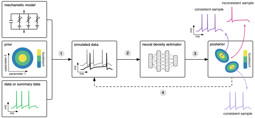
Central to many questions in neuroscience is how signal changes relate to underlying neural mechanisms during particular cognitive tasks. In general a hypothesis about the underlying mechanism is cast into a mechanistc or probabilistic model and some free parameters are optimized to fit the empirical data. Several issues come up with standard Bayesian inference methods: the full training procedure has to be performed for each source of data that one wants to infer, and the uncertainty and interactions between parameters remain unknown. For these reasons among others simulation based inference (SBI) methods are developed (sometimes called Generalized Bayesian Inference (GBI)). Here you have a similar unknown black-box mechanistic model (can be non-linear and highly complex), meaning the internal mechanisms are not accessible and do not have to be differentiable. The black-box model is only required to take a set of parameters ($\theta$) and generate a set of observations ($\psi$). In this way we can formulate this black-box mechanistic model as an unknown function ($F$):

$\psi = F_{\theta}(x)$

Where $F$ is conditioned on the free parameters ($\theta$, e.g. connectivity), and $x$ are the experimental factors such as stimulus onset and duration (i.e. parameters which are not of interest for inversion). Taking a set of samples from a prior distribution $p(\theta)$ of the parameters of interest one can run a number of simulations ($N$) and obtain a dataset containing the instantiations of the parameters and the resulting observations ($[\theta_i,\psi_i]_{i=1}^N$). This dataset is then a set of samples taken from:

$p(\theta,\psi)=p(\theta)p(\psi,\theta)$

This dataset can be used to train a neural density estimator (specific kind of deep neural network for training distributions instead of classes) which will learn the distribution which quantifies the relationship between parameters and observations. We can apply new observation data to this distribution and infer an approximation of the posterior $p(\theta,\psi_{new})$. In other words, we can approximate the set of parameters given a new set of observations. This methods allows for amortized inference afeter the training procedure is complete (i.e. simulations of the model are only run to obtain the dataset, after training simulating is not required anymore).

Inference of the Lorenz System

To show the power of neural networks in learning distributions, and thus of underlying model parameters given some set of training data, I will show some results of the method applied to the Lorenz System. The Lorenz System is a simple model with three variables and a few parameters but exhibits very chaotic dynamics. It is therefore a good model to test the approach with. The Lorenz model is defined as follows:

$\begin{align*} \frac{dx}{dt} &= \sigma (y - x) \\ \frac{dy}{dt} &= x (\rho - z) - y \\ \frac{dz}{dt} &= x y - \beta z \end{align*}$

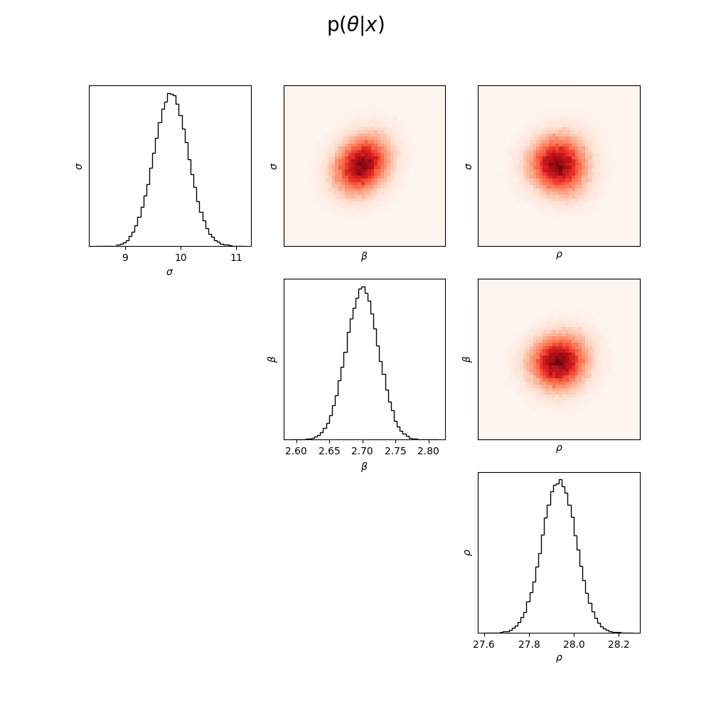
The Lorenz system has 3 parameters ($\sigma$, $\beta$, and $\rho$), 3 variables ($x$, [y]($mathtex, and $z$. I use a set of summary statistics (mean, covariance, correlation, eigvalues, lyapunov exponents) which are generated by running the model with a bunch of times with a lot of different parameters and initial conditions (e.g. 10000 simulations). These I fed into a density estimator together with the parameters. The neural network then learned the relation between the summary statistics and the parameters.

Hopefully the application becomes clear when we turn the problem on it’s head and perform inference. For example, I generate some data by running a single simulation of the model with parameters $\sigma = 10$, $\beta = \frac{8}{3}$, and $\rho = 28$. Then this data is given to the neural network whose parameters now generate distributions from which I can take a number of samples (e.g. 1000 samples). If I then plot these density of the samples, which are now in the parameter space you can easily see that the neural network returns values very close to the ground truth.

This is a toy example, but not a trivial one. The Lorenz system has chaotic dynamics which are common in a lot of systems found in nature. The ability to infer parameters from systems from which we can only measure chaotic and unpredictable observations is very interesting. In a follow-up post I will dive into how the same technique can be applied to infer neural activations from brain activity measurements.

Notes

• The search space grows very fast with the number of parameters that are of interest for the inference.
• The quality of the inference depends heavily on the quality and diversity of the simulations used for training.
• Choosing appropriate summary statistics is crucial for the performance of the neural density estimator.
• It is important to validate the trained model with independent test data to ensure its generalizability.
• Hyperparameter tuning of the neural network can significantly impact the accuracy of the inferred parameters.
• Visualization of the inferred parameter distributions can provide insights into the uncertainty and (marginal) correlations between parameters.

The code for this little experiment is publicly available on GitHub.

References

1. Papamakarios, G., Nalisnick, E., Rezende, D. J., Mohamed, S., & Lakshminarayanan, B. (2019). Normalizing Flows for Probabilistic Modeling and Inference. Journal of Machine Learning Research, 22(57), 1-64.
2. Cranmer, K., Brehmer, J., & Louppe, G. (2020). The frontier of simulation-based inference. Proceedings of the National Academy of Sciences, 117(48), 30055-30062.
3. Lorenz, E. N. (1963). Deterministic nonperiodic flow. Journal of the Atmospheric Sciences, 20(2), 130-141.